The term "behavioral data" and its benefits for market research may not be new for most of you. One of the most prominent features of this sort of information is that the data acquired is independent of the memory capabilities and social desirability of our participants, which makes it stand over declarative data whenever a more objective perspective is needed. Particularly online behavioral data has become very popular nowadays because of the wide range of possibilities it has to offer.
We can all easily grasp the intuitive idea that inspecting the domains we visit online, the order in which we do so, and what we do on each domain can be very valuable information for market research. One can find hundreds of posts and online speeches on what can be done with this sort of data and the relevance of such data. However, most of them only cover the topic at a very high level, without really getting into it, leaving the technical part aside. Then, even though we may have a clear goal we want to reach, we might find ourselves wondering how we can explicitly use our data to answer the kind of questions we need answers for.
This blog post aims to outline a simple analysis that goes from a bunch of online behavioral data to a set of conclusions we can later use to make informed decisions. Concretely, we’ll use a data set of online visits to museum-related websites as an example. From this data set, we’ll learn which are the websites with more visits, which is the profile of those visitors, who purchased tickets online, and the profile of those online buyers. Results of this analysis can be crucial before launching a marketing campaign, since it allows to segregate according to the interests of the different groups.
You might be wondering where we can get this data from. Netquest is a market research company that does not only deliver online surveys to their panelists, but those who are invited and give us informed consent are passively metered. All they have to do is to install the meter on the devices they want, and it will send us their online activity from that device. For the purposes of this blog post, we collected all the records associated to museoreinasofia.es (Museo Reina Sofía, Madrid), sagradafamilia.org (Sagrada Familia, Barcelona), patrimonionacional.es (Patrimonio Nacional, Spain) and cac.es (Ciutat de les Arts i les Ciències, València). That
data came from the panel in Spain in 2017, it was formed of 11,088 observations and it involved 722 panelists. The analysis and the plots were carried out in R. Before diving into the analysis, we need to describe our data set more thoroughly.
An online behavioral data set
Every time panelists load a website, there is a set of variables which unambiguously pinpoint that online visit among the set of online behavioral data. This data must necessarily involve the URL of access, the timestamp, the device used and who performed that online access. We may think this is already sufficient to determine any online visit, however, for the sake of simplicity of the analysis, we decided to add the domain name of the URL. Such variable can readily tell us whether a panelist is navigating within the same domain, or he/she is jumping from domain to domain, without the need for manipulating the URL.

First insight: counting visits
The domain name variable may suggest the first piece of analysis: we can group the online visits to the same domain altogether and count how many we can find for each group. This will tell us how many times each website is visited. Now, if we also sort this data, we can generate a ranking of popularity of all the domains considered in our data set.
Let’s use our museum data set, grouped by domain name and have a look at what we get:
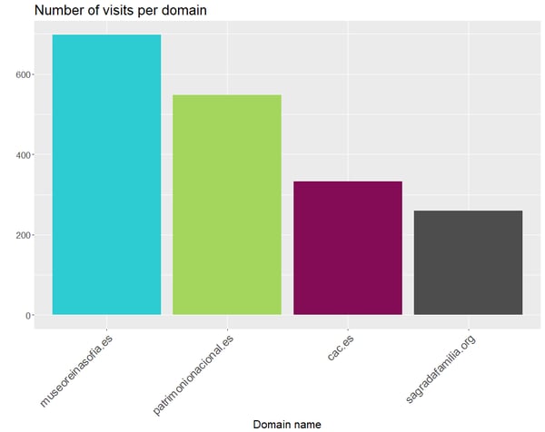
We can clearly see that the museum with the largest number of visits is Museo Reina Sofía. A possible explanation may be that this museum changes their art exhibit periodically, what may encourage visitors to go to their website quite often to see what’s new.
If we use this kind of analysis, we will learn the relative popularity of our website among the others in the field. To this aim, the list of domains should be formed of our own website and our direct competitors, so that the final ranking tells us how popular we are in respect to the others.
Who are those visitors?
A quite common wonder is who is visiting the websites we need to analyze. Having that information will allow us to:
- Know the users of each website, which we can use to improve retention
- Find discrepancies between our expected target population and the real audience, so that we can launch targeted marketing campaigns to those specific groups
- Find potential new users among those who already visit similar websites to ours
The idea behind this analysis is to group by domain name again, and to aggregate the personal details of the people who accessed each domain, since that will give us a profile of its visitors. However, we don’t have that information on our data set. What we do have is a variable storing who performed each of the online visits, the panelist ID. On the other hand, since those visitors are Netquest panelists, we have tones of personal data we can use, and their associated to a panelist ID too. Then, all we need to do is to match the IDs of the panelists, and to add the personal details to our original data set. Consequently, each observation in the merged data set will include the URL accessed, the timestamp, the device used, the domain name, who performed that online visit, in addition to all the personal details we need to form the users profile. We can now group that data grouping by domain name and get percentages of each of the features of the users. Thus, we will have built a profile of the users of each domain with very little effort.
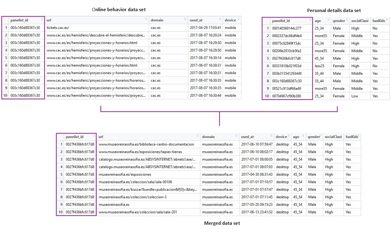
Now we can go back to our example data set and perform that merge. To get the visitor profile, we will only include the variables gender, social class, the number of kids and whether they read the press or not. Once it’s done, we group by domain name and calculate the percentages of each possible value in the variables included. For instance, in the case of the variable gender, we’ll calculate the percentage of women and the percentage of men. We’ll do the same for the remaining variables.
Results can be found below:
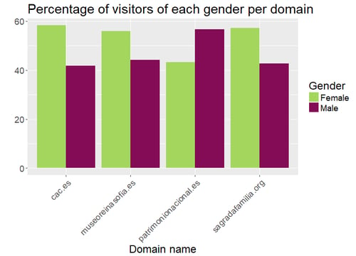
![]()
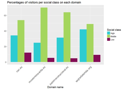
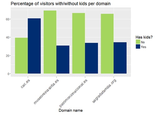
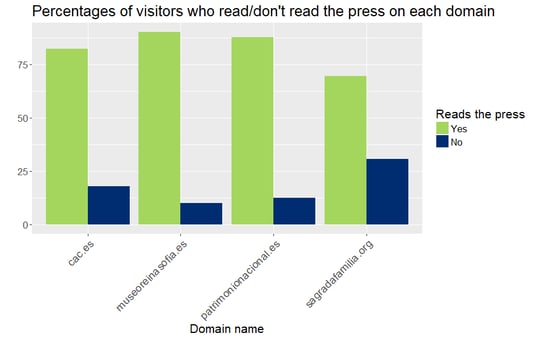
We can observe no critical difference between the percentages of men and women who visited these websites. However, we did find differences regarding the other three variables. The social class is clearly indicating that the middle social class visits these websites more often than the high class and the low class. The variable indicating whether the users have kids is suggesting that the Ciutat de les Arts i les Ciències may be more children-friendly than the other three options. And finally, most visitors to museum-related websites read the press.
Intuitively, we may think that adding information about the visitors is the only way we can get their profile; nevertheless, online behavioral data itself can suggest user habits. If we split the timestamp data into time frames (eg. early morning, morning, afternoon, and night), and aggregate this data per domain, we will learn when users preferably access those websites. The same procedure can be followed to get the month of access to those websites, which we can use to learn the yearly behaviour of users. From this, we can learn whether it is a periodic behaviour or it varies every year; and if we have historic data, this may also help us detect potential technical issues due to drastic drops in the number of visits.
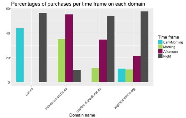
We generated the new variable time_frame for our example. We decided to split the timestamp information into 4 time periods: Early morning (00-06h), morning (06-12h), afternoon (12-18h), and night (18-00h). After grouping by domain and aggregating the
data into percentages, we obtained the following results:
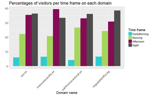
As we can see, most online users access these websites either during the afternoon or at night, and few of them do it in the morning.
Do people purchase on these websites?
We might also wonder whether users bought anything on these websites, and if so, how we can describe these online buyers. However, detecting online purchases among a set of online behavioral data is not straightforward. We need to know the purchase
confirmation URL beforehand, which can be either provided by the client or we may need to find it ourselves, which can be tedious work. But once we know them, we can detect purchase URLs using regular expressions, and flag all the observations we find. If we gather these visits and we count how many there are per domain, we will get the total amount of purchases per website. And that’s exactly what we did with our example data set. The table with the summary of the number of visits and the number of users per domain can be found below:
| Domain name | Number of Purchases | Number of users who purchased |
| museoreinasofia.es | 7 | 3 |
| sagradafamilia.org | 6 | 6 |
| patrimonionacional.es | 2 | 2 |
| cac.es | 1 | 1 |
Finally, we can generate a profile of those online buyers by including the personal details we used earlier before and aggregating them by domain name following the same procedure. We generated simple profiles with the variables age and time_frame:
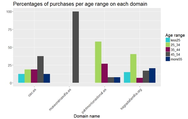
Online buyers of the websites patrimonionacional.es and sagradafamilia.org are more likely to be aged [25, 34]. Those of the domain museoreinasofia.es are bound to be aged [45, 55], while those from cac.es are quite spread in terms of age. And regarding the time frames when those purchases were carried out, it seems that preferable times are night time and afternoon. Even though half of the purchases on cac.es happened on the early morning time frame, it seems to be the continuation of the night time. This is coherent with the previous analysis, where we learnt that users preferably visit at the afternoon or at night.
Conclusions and further analysis suggestions
The analysis reported in this post is extremely simple, since it’s only based on gathering all the data together according to their domain name, and aggregating it to obtain a description of the online visits/purchases and the users of each domain. However, despite being that simple, it already provided a lot of valuable information we can use to make several informed decisions.
More complex analysis can be run over such data to gain other kinds of insight. Here are some of the possibilities (with possible uses):
- Clustering the visitors to specific websites: a segmentation of the target population will allow us to launch directed campaigns to our target population organized in groups. Such segmentation can be built following any criteria: sociodemographic data, reasons to visit the website, personal interests, and so on
- Prediction of purchases: a predictive model that indicates when users are more likely to buy specific products may help us organise the website
- Finding probabilities of new registrations: finding out who are those potential users with the highest probability of becoming new users may allow us to save a lot of money
- Recommender system: this will suggest products users may be interested in buying, which may increase the total count of online purchases