In an earlier post, we saw the definition, advantages and drawback of simple random sampling. Today, we’re going to take a look at stratified sampling.
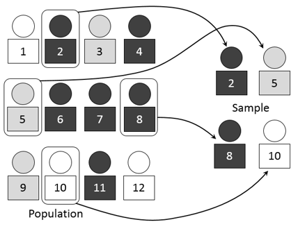
This method, which is a form of random sampling, consists of dividing the entire population being studied into different subgroups or discrete strata (the plural form of the word), so that an individual can belong to only one stratum (the singular). Once the strata have been defined, in order to create a sample, we select individuals by applying a sampling method to each of the strata separately. If, for example, we use simple random sampling for every stratum, we’re using what’s called stratified random sampling (StratRS). We can also use other sampling methods for every stratum, such as systematic sampling and random sampling with replacement.
Strata tend to be homogeneous groups of individuals, while groups are heterogeneous among themselves. For example, if we’re expecting very different behavior between men and women in a study, it would be convenient to define two strata, one for each gender. If we have selected these strata correctly, (1) men should behave similarly to each other, (2) women should behave similarly to each other and (3) men and women should exhibit dissimilar behavior.
If this condition (strata are internally homogeneous and heterogeneous among themselves) is met, then using StratRS reduces sampling errors and improves the precision of our results when we base a study on our sample.
It is fairly common to define strata based on certain variables that are characteristic of the population, such as age, sex, class or geographic region. These variables make it easy to divide the sample into mutually exclusive groups and enable us to discern different behaviors within the population.
Types of stratified sampling
Depending on the size that we assign to the strata, we can talk about different sorts of stratified sampling. It’s also common to talk about different ways of “allocating” the sample into strata.
(1) Proportional stratified sampling
When we select a characteristic of the individuals in order to define the strata, the resulting subpopulations are often different sizes. Let’s say that we want to study the percent of the Mexican population that smokes, and we decide that age would be a good criterion to stratify (that is, we think that smoking habits might vary significantly by age). We define three strata: under twenty, twenty to forty-four and forty-five and up. When we divide the population of Mexico into these three strata, we don’t expect all three groups to be the same size. And, in fact, the real data confirm this:
* Stratum 1 - Mexican population younger than twenty: 42.4 million (41.0%)
* Stratum 2 - Mexican population between twenty and forty-four: 37.6 million (36.3%)
* Stratum 3 - Mexican population older than forty-four: 23.5 million (22.7%)
If we use proportional stratified sampling, the sample should consist of strata that maintain the same proportions as the population. If, for this example, we want to create a sample of 1,000 individuals, the strata must have the following sizes:
| Stratum | Population | Proportion | Sample |
| 1 | 42,4M | 41,0% | 410 |
| 2 | 37,6M | 36,3% | 363 |
| 3 | 23,5M | 22,7% | 227 |
2) Uniform stratified sampling
We talk about uniform allocation when we assign the same sample size to all of our defined strata, regardless of those strata’s weight within the population. A uniform stratified sampling of the above example would yield the following sample for each stratum:
| Stratum | Population | Proportion | Sample |
| 1 | 42,4M | 41,0% | 334 |
| 2 | 37,6M | 36,3% | 333 |
| 3 | 23,5M | 22,7% | 333 |
This method favors strata that have less weight in the population by affording them the same level of importance as the more relevant strata. This reduces the global effectiveness of our sample (the results will be less precise), but it enables us to study individual characteristics of each stratum with greater precision. In our example, if we want to make some specific statement about the population of Stratum 3 (those older than forty-four), we could reduce sampling errors by using a 333-unit sample, rather than a 227-unit sample (which we would use in proportional stratified sampling).
(3) Optimal stratified sampling (with respect to standard deviation)
In this case, the size of the strata in the sample is not proportional to the population. Rather, the size of the strata is proportional to the standard deviation of the variables being studied. In other words, the strata with the greatest internal variability are the largest, so that the whole sample better represents the groups that are most difficult to study.
Effectiveness of different stratified samplings
The inevitable questions are: When is it best to use stratification? Which kind of stratification is best?
- Proportional stratified sampling always produces the same number of sampling errors as simple random sampling, or fewer. This means that it is more precise. We achieve equality when the averages or proportions that we are studying are equal in all strata. Therefore, stratification is more beneficial when the strata are more diverse among themselves.
- Optimal stratified sampling is always as precise or more precise than proportional stratified sampling. These methods are equally precise and totally equivalent when the typical variations within each stratum are equal. Therefore, optimal stratification is more beneficial when there is greater variation within each group, a situation in which we could reduce the sample size of the most homogeneous group and favor those that are more heterogeneous. Then again, this is a more complex method that requires a lot of information about the sample before we even get started—information that we often don't possess.
Sample sizes required for each method
Now we've seen how stratification can be beneficial. Not only can these methods be used to more precisely estimate averages (e.g. the average number of cigarettes consumed by smokers in Mexico) and proportions (e.g. the percent of the Mexican population that smokes); they also enable us to reduce the sample size necessary to make an estimate with a predetermined level of error.
The table below summarizes the sample size required for each method, based on the maximum level of error that we are willing to accept and the characteristics of the population itself, which we will assume is infinite in size (if it is finite, a correcting factor must be applied).

To understand the above table, you have to know that:
- Z = The deviation from the mean value that we will accept in order to achieve our desired confidence level. Depending on the confidence level we want, we'll use a cutoff value based on the quantiles of the Gaussian distribution. The most common values are:
90% confidence level -> Z=1.645
95% confidence level -> Z=1.96
99% confidence level -> Z=2.575
- L is the number of strata into which we divide the sample and h represents a particular stratum. Therefore, h can vary between 1 and L strata.
- p is the proportion of the total population that we are trying to determine (e.g. the percent of the Mexican population that smokes). Therefore, (1-p) is the complementary proportion of the population; that is, the proportion of the population to which the sought criterion does not apply (non-smokers). Likewise, ph represents that proportion within each stratum.
- σ2 is the variance of the data we’re seeking (in the case of estimating averages) within the total population. σh2 is the variance within every stratum.
- e is the accepted margin of error.
- Wh is the stratum’s weight within the sample (the size of the stratum with respect to the whole sample). If we’re talking about proportional stratification, every Wh is equal to the proportion represented by that stratum in the population. If we’re talking about optimal stratification, every Wh is calculated based on the dispersion within each stratum.
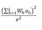
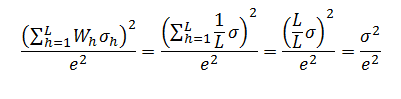
Using the formulas above, it is possible to demonstrate that these different stratification methods only reduce the sample size if the values p and σ vary between strata. Otherwise, all of the expressions are equivalent. Let’s take a look at an example: if we take the expression of sample size required to estimate an average by means of optimal stratified sampling (ignoring the parameter Z in this case)
and we consider all of the strata’s variances to be equal (σh=σ) and further consider the strata to be identical in size (Wh=1/L), we get
We hope that this post has helped clarify how useful stratified sampling can be. In our next few posts, we’ll tackle systematic sampling.
TABLE OF CONTENTS: Series on sampling
- Sampling: What it is and why it works
- Random and non-random sampling
- Random sampling: Simple random sampling
- Random sampling: Stratified sampling
- Random sampling: Systematic sampling
- Random sampling: Cluster sampling
- Non-random sampling: Availability sampling
- Non-random sampling: Quota sampling
- Non-random sampling: Snowball sampling